•  Home
  •  Topics 
    •  Solar Physics
    •  Planetary atmospheres
    •  Stellar environments
    •  Star-planet interactions
    •  Stellar physics
    •  Star formation
    •  Interstellar medium
    •  Supernovae
    •  Galactic dynamics
    •  Cosmology
  •  About Galactica
  •  Publish my projects
  •  Share massive data
  •  Log in
Extreme Horizon

Extreme Horizon

Resolving galactic disks in their cosmic environment

Orion

Orion

Molecular cloud fragmentation and evolution, formation of prestellar cores

Fragdisk

Fragdisk

Fragmentation of self-gravitating disks

Synthetic disk populations

Synthetic disk populations

Resolving protoplanetary disks in massive protostellar clumps

Wind of HD189733

Wind of HD189733

Unveiling the magnetic link between stars and planets

Dusty collapses

Dusty collapses

Understanding the dynamics of dust during the protostellar collapse

Previous Next
  1. Home
  2. Cosmology
  3. Extreme Horizon
  4. Extreme Horizon (50 Mpc run)

Acknowledgement

Project acknowledgement

To acknowledge this project, please cite :

               @ARTICLE{2020A&A...643L...8C,
                   author = {{Chabanier}, S. and {Bournaud}, F. and {Dubois}, Y. and {Codis}, S. and {Chapon}, D. and {Elbaz}, D. and {Pichon}, C. and {Bressand}, O. and {Devriendt}, J. and {Gavazzi}, R. and {Kraljic}, K. and {Kimm}, T. and {Laigle}, C. and {Lekien}, J. -B. and {Martin}, G. and {Palanque-Delabrouille}, N. and {Peirani}, S. and {Piserchia}, P. -F. and {Slyz}, A. and {Trebitsch}, M. and {Y{\`e}che}, C.},
                   title = "{Formation of compact galaxies in the Extreme-Horizon simulation}",
                   journal = {\aap},
                   keywords = {galaxies: formation, galaxies: evolution, galaxies: high-redshift, galaxies: structure, methods: numerical, Astrophysics - Astrophysics of Galaxies},
                   year = 2020,
                   month = nov,
                   volume = {643},
                   eid = {L8},
                   pages = {L8},
                   doi = {10.1051/0004-6361/202038614},
                   archivePrefix = {arXiv},
                   eprint = {2007.04624},
                   primaryClass = {astro-ph.GA},
                   adsurl = {https://ui.adsabs.harvard.edu/abs/2020A&A...643L...8C},
                   adsnote = {Provided by the SAO/NASA Astrophysics Data System}
               }

Galactica database acknowledgement

If you use it in your own work, you may acknowledge the origin of the data obtained on the Galactica database like so:

This work reused datasets available on the Galactica simulations database
(http://www.galactica-simulations.eu)
                            
Cite me
Frédéric BOURNAUD  

Extreme Horizon (50 Mpc run)

  • Summary
  • Parameters
  • Algorithms
  • Applied physics
  • Results
    • Stellar mass distribution
  • Snapshots
    • t=$0.2$
    • t=$0.25$
    • t=$0.333333$

Summary

The Extreme Horizon simulation (EH) is performed with the adaptive mesh refinement code RAMSES (Teyssier 2002) using the physical models from Horizon-AGN (Dubois et al. 2014). The spatial resolution in the CGM and IGM is largely increased compared to Horizon-AGN, while the resolution inside galaxies is identical, at the expense of a smaller box size of $50 \; \textrm{Mpc}\cdot\textrm{h}^{-1}$. The control simulation of the same box with a resolution similar to Horizon-AGN is called Standard-Horizon (SH). EH and SH share initial conditions realized with mpgrafic (Prunet et al. 2008). These use a $\Lambda\textrm{CDM}$ cosmology with matter density $\Omega_{\textrm{m}} = 0.272$, dark energy density $\Omega_{\Lambda} = 0.728$, matter power spectrum amplitude $\sigma_{8} = 0.81$, baryon density $\Omega_{\textrm{b}} = 0.0455$, Hubble constant $\textrm{H}_{0} = 70.4 \; \textrm{km}\cdot\textrm{s}^{-1}\cdot\textrm{Mpc}^{-1}$, and scalar spectral index $\textrm{n}_{\textrm{s}} = 0.967$, based on the WMAP-7 cosmology (Komatsu et al. 2011). The Extreme Horizon simulation was performed on 25 000 cores of the AMD-Rome partition of the Joliot Curie supercomputer at TGCC and it partly used the Hercule parallel I/O library (Bressand et al. 2012; Strafella & Chapon 2020). It is being run down to $z\simeq 1.0$.

Resolution strategy

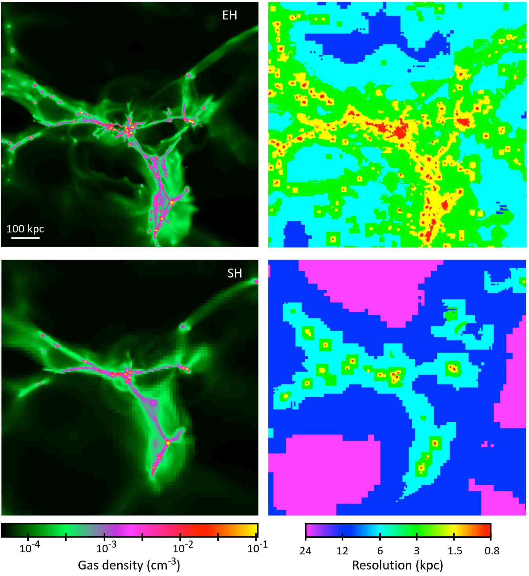
The Standard-Horizon simulation uses a $512^{3}$ coarse grid, with a minimal resolution of $100 \; \textrm{kpc}\cdot\textrm{h}^{-1}$ as in Horizon-AGN. Cells are refined up to a resolution of $\simeq 1\; \textrm{kpc}$ in a quasi-Lagrangian manner: any cell is refined if $\rho_{\textrm{DM}} \Delta\textrm{x}^{3} + (\Omega_{\textrm{b}}/\Omega_{\textrm{DM}})\rho_{\textrm{baryon}}\Delta x^{3} > \textrm{m}_{\textrm{refine},\textrm{SH}}\textrm{M}_{\textrm{DM},\textrm{res}}$, where $\rho_{\textrm{DM}}$ and $\rho_{\textrm{baryons}}$ are dark matter (DM) and baryon densities respectively in the cell, $\Delta x^{3}$ is the cell volume, and $\textrm{m}_{\textrm{refine},\textrm{SH}}=80$. The $\Omega_{\textrm{b}}/\Omega_{\textrm{DM}}$ factor ensures that baryons dominate the refinement condition as soon as there is a baryon overdensity. This resolution strategy matches that of Horizon-AGN :
The first two lines indicate the comoving and physical (at $z=2$) grid resolution in $\textrm{kpc}\cdot\textrm{h}^{-1}$ and $\textrm{kpc}$, respectively. The last three lines indicate the volume fractions measured at each resolution level at $z=2$ in EH, SH and HAGN for comparison. In the last two columns, $z<2$ means that these levels are not triggered yet at $z=2$ but will be for lower redshifts.
Comoving grid resolution $[\textrm{kpc}\cdot\textrm{h}^{-1}]$ 97.6 48.8 24.4 12.2 6.1 3.05 1.52 0.76
Physical grid resolution [kpc] ($z=2$) 47 23.5 11.7 5.8 2.9 1.5 0.7 0.3

Volume fraction (EH) ($z=2$) - 45% 43% 10% 1% 0.04% $z<2$ $z<2$
Volume fraction (SH) ($z=2$) 80% 17% 2% 0.17 % 0.013% $5\times10^{-4} %$ $z<2$ $z<2$
Volume fraction (HAGN) ($z=2$) 77% 19% 2% 0.2 % 0.01% $6\times10^{-4} %$ $z<2$ $z<2$

The Extreme Horizon simulation uses a $1024^{3}$ coarse grid and a more aggressive refinement strategy with $\textrm{m}_{\textrm{refine},\textrm{EH}}=1/40 \, \textrm{m}_{\textrm{refine},\textrm{SH}}$ in the IGM/CGM (for $\Delta x > 1.52 \; \textrm{kpc}\cdot\textrm{h}^{-1}$), but with $\textrm{m}_{\textrm{refine},\textrm{EH}}=\textrm{m}_{\textrm{refine},\textrm{SH}}$ near to and in galaxies: the whole volume is resolved with a resolution that is twice as high and most of the mass is resolved with a four times higher resolution in 1D, yielding an improvement of 8 to 64 for the 3-D resolution. This improvement continues until the highest resolution of $\simeq1 \; \textrm{kpc}$ is reached. Such an aggressive approach for grid refinement can better model the early collapse of structures (O'Shea et al. 2005). Appendix A illustrates the resolution achieved in representative regions of the CGM and IGM in EH and SH. The resolution in EH haloes is typically $\sim 6\; \textrm{kpc}$, while it is $\sim 25\;\textrm{kpc}$ for SH. However, galaxies themselves are treated at the very same resolution in EH and SH: any gas denser than $0.1 \; \textrm{cm}^{-3}$ is resolved at the highest level in SH, as is also the case for 90% of the stellar mass.

Baryonic physics

Like in Horizon-AGN (Dubois et al. 2014), reionization takes place after a redshift of 10 due to heating from a uniform UV background from Haardt & Madau (1996). There is H and He cooling implemented as well as metal cooling, following the Sutherland & Dopita (1993) model.

Star formation occurs in cells with a hydrogen number density larger than $\rho_{0}=0.1 \; \textrm{H}/\textrm{cm}^{3}$. The star formation rate density is $\dot{\rho_{*}} = \epsilon_{*}\textrm{t}_{\textrm{ff}}$, where $\textrm{t}_{\textrm{ff}}$ is the local gas free-fall time and $\epsilon_{*}=0.02$ is the star-formation efficiency (Kennicutt 1998). Mass, energy, and metals are released by stellar winds, with type Ia and type II supernovae, assuming a Salpeter Initial Mass Function.

Black holes (BH) are represented by sink particles with an initial mass of $10^{5} \; \Msun$. They accrete gas through an Eddington-limited Bondi-Hoyle-Lyttleton model. Boosted accretion episodes are included when the gas density overcomes a density threshold aimed at mitigating resolution effects, with the boosting calibrated to produce realistic BH masses. The AGN feedback comes in two modes (Dubois et al. 2012): the quasar mode injects thermal energy and the radio mode injects mass, momentum, and kinetic energy into the surrounding medium. For a detailed parameterization of these models, we refer to Dubois et al. (2014), the analysis of Dubois et al. (2016), and Dubois et al. (2012).

Simulated using Ramses 3

Parameters

Parameter Value
$\textrm{H}_{0}$ $70.4 \; \textrm{km}\cdot\textrm{s}^{-1}\cdot\textrm{Mpc}^{-1}$
$\Omega_{m}$ $0.272 \; $
$\Omega_{\Lambda}$ $0.728 \; $
$\Omega_{b}$ $0.04455 \; $
$\sigma_{8}$ $0.81 \; $
$\textrm{n}_{s}$ $0.967 \; $
box size $50 \; \textrm{Mpc} \cdot \textrm{h}^{-1}$
Lmin $10 \; $
Lmax $16 \; $
$\epsilon_{*}$ $2 \; \%$
$\rho_{0}$ $0.1 \; \textrm{H}/\textrm{cc}$

Algorithms

Adaptive mesh refinement
RAMSES octree AMR implementation [Teyssier 2002]
Harten-Lax-van Leer-Contact Riemann solver
Riemann solver implementation [Teyssier 2002]

Applied physics

Star formation
Star formation specific implementation [Teyssier 2002]
Self-gravity
Self-gravity implementation details ([Teyssier 2002], [Guillet and Teyssier 2011])

Results

'Stellar mass distribution' generic result datafile download

Select the datafiles you wish to export from this generic result (a zip file containing the requested datafiles will be prepared) :

Stellar mass distribution

There are 37 698 galaxies detected in Extreme Horizon at $z\sim2$ and 20 314 in Standard Horizon, with stellar mass functions attached below. While the mass functions above $10^{10} \; \Msun$ are quite similar in both simulations, Extreme Horizon forms twice as many galaxies as Standard Horison with stellar mass $\textrm{M}_{*} \le 5\times 10^{9} \; \Msun$. We rule out any detection bias since stellar particles have similar masses in both simulations (new stars form at the maximal resolution level in each simulation) and we attribute this difference to the increased resolution in low-density regions. Fitting the $z=2$ mass function with a power law of the form $\Phi(\textrm{M}_{*}) \propto \textrm{M}_{*}^{\beta}$ in the $10^{9} \le \log(\textrm{M}_{*}/\Msun) \le 10^{9.5}$ range yields $\beta \simeq -0.68$ for Extreme Horizon and $-0.34$ for Standard horizon. Observations indicate a slope of $-1.0 \le \beta \le -0.5$ in this mass range ( Santini et al. 2012; Tomczak et al. 2014), demonstrating that low-mass galaxy formation is substantially under-resolved or delayed in Standard Horizon.
Datafiles:
Stellar mass functions
Number of galaxies per mass bin in Extreme Horizon and Standard Horizon at $z = 2$, $3$, and $4$.
  • PNG 

Snapshots

$Z \sim 4$ (t=$0.2$)

Simulation snapshot at redshift $Z \simeq 4$
Catalogs :
  • Galaxy catalog (7693 galaxy objects)

'$Z \sim 3$' snapshot datafile download

Select the datafiles you wish to export from this snapshot (a zip file containing the requested datafiles will be prepared) :

$Z \sim 3$ (t=$0.25$)

Simulation snapshot at redshift $Z \simeq 3$
Catalogs :
  • Galaxy catalog (24704 galaxy objects)
Datafiles:
Gas density in the CGM and IGM around a massive halo in the Extreme Horizon and Standard Horizon simulations in the same region.
Projected density (left) and physical resolution (right) in Extreme Horizon (top) and Standard Horizon (bottom) zoomed on a massive halo at $z=3$. The depth of the projections are $200 \; \textrm{kpc}\cdot\textrm{h}^{-1}$ and the boxes extend to $1 \; \textrm{Mpc}\cdot\textrm{h}^{-1}$ on each side. The gas density is computed as the mass-weighted average of local densities along the line of sight corresponding to each pixel. The resolution shown is the resolution of the cell in which the gas density is the highest along each line of sight.
  • PNG 

'$Z \sim 2$' snapshot datafile download

Select the datafiles you wish to export from this snapshot (a zip file containing the requested datafiles will be prepared) :

$Z \sim 2$ (t=$0.333333$)

Simulation snapshot at redshift $Z \simeq 2$
Catalogs :
  • Galaxy catalog (37698 galaxy objects)
  • Ultra-compact galaxy catalog (10 galaxy objects)
Datafiles:
Large-scale structure of the Extreme Horizon simulation at redshift $z = 2$
Projected map of the EH simulation at $z \simeq 2$. Gas density (grey), entropy (red), and metallicity (green) are shown.
  • PNG 

 Go to top

This material is Open Data